Final progress update
First, a brief aside: if you were directed here from the GSoC project list, you might want to check out the rest of my blog for some more background info first!
So, GSoC 2018 is coming to an end…
I had an amazing time this summer with GSoC, full of challenges and surprises, and I am grateful for everyone’s support and encouragement.
Special thanks go out to my mentor Simon Danisch (@SimonDanisch) for bearing with me and being such an excellent mentor!
The main working goals of my project are:
- Extending the documentation and documentation capabilities of
Makie.jl - Implement database reference queries in the documentation pages
- Improve current documentation
- Implement additional plot examples
- Implement overview pages for the plotting functions, including examples
- Implement plots collage image for categorical pages (e.g. collage of all scatter plots)
- Implement preview gallery / categorical pages of plot types (e.g. all scatter plots)
- Automate the documentation generation
The following is a summary of what was achieved for Makie.jl. Note that Makie.jl implements a higher-level layer to the AbstractPlotting.jl package (also by Simon), which provides the atomic plotting functions that enable plotting.
Extending the documentation capabilities
Various help functions were implemented: help, help_arguments and help_attributes.
These can be used as such:
julia> help(scatter; extended=true)

`scatter(x, y, z)` / `scatter(x, y)` / `scatter(positions)`

Plots a marker for each element in (x, y, z), (x, y), or positions.

AbstractPlotting.scatter has the following function signatures:

  (Vector, Vector)
  (Vector, Vector, Vector)
  (Matrix)

Please refer to convert_arguments to find the full list of accepted arguments

Available attributes and their defaults for Scatter{...} where T are:

  alpha             1.0
  color             :black
  colormap          :viridis
  colorrange        AbstractPlotting.Automatic()
  glowcolor         RGBA{N0f8}(0.0,0.0,0.0,0.0)
  glowwidth         0.0
  linewidth         1
  marker            GeometryTypes.HyperSphere{2,T} where T
  marker_offset     AbstractPlotting.Automatic()
  markersize        0.1
  rotations         AbstractPlotting.Billboard()
  strokecolor       RGBA{N0f8}(0.0,0.0,0.0,0.0)
  strokewidth       0.0
  transform_marker  false
  visible           true

You can see usage examples of AbstractPlotting.scatter by running:

example_database(AbstractPlotting.scatter)
There were backend changes that were necessary to implement these help functions, such as the collection, iteration and pretty-printing of the plots attributes dictionaries, and the type conversions necessary to handle function handle or Plot type inputs, etc.
Implement database reference queries in the documentation pages
A custom extension in Documenter’s Selectors.matcher and Selectors.runner was implemented to use regex-matching on strings of the form
@example_database("scatter example", plot).
Then, during the compilation of the documentation using Documenter.makedocs(), Documenter will automatically insert the plot of the specific example into the document at the correct place.
This is done by overloading the runner to write custom HTML embed code for the plots.
For animated plots, the embed code is able to embed the animations (either as .gif, or .mp4).
Furthermore, one can write @example_database("plot example", code) to embed just the source code of the example (more on this later). Likewise, @example_database("plot example", stepperplot) embeds plots from Stepper examples, and @example_database("plot example") embeds both the plot, plus the source code.
Improve current documentation
Various quick-start guides and tutorials were added to the documentation (now visible online at https://makie.juliaplots.org/stable/) to help first-time users get started quickly with Makie.
A landing page was added as well, which serves as the index page of the online docs. This is intended to offer a brief showcase for some of the plots that can be made using Makie.
In addition, detailed documentation pages about the help functions, atomics plotting functions, plot signatures and attributes, axis theming, interaction (including animation of plots), and output (saving) of plots were added.
Implement additional plot examples
Many plots were implemented throughout the entire GSoC coding period, utilizing the various atomics plotting functions.
Some of the plots were created as part of the tutorials (e.g. to show how to theme a plot, or animate a plot), or as example pieces for the documentation pages (e.g. to show how to output an animated plot to a file). Some of the examples are created to showcase the customization capabilities of the plotting commands, such as the extensive theming options, text annotations, colormaps options, etc.
Animated plots were also created. Some plot examples that could be more applicable to scientific contexts were created. Some “meta” plots were created that showed some Makie internals, such as the plots that showed the available gradients for colormaps, or the available marker symbols for scatter plots. And some plots were created to the plotting of implicit functions in 2D and 3D.
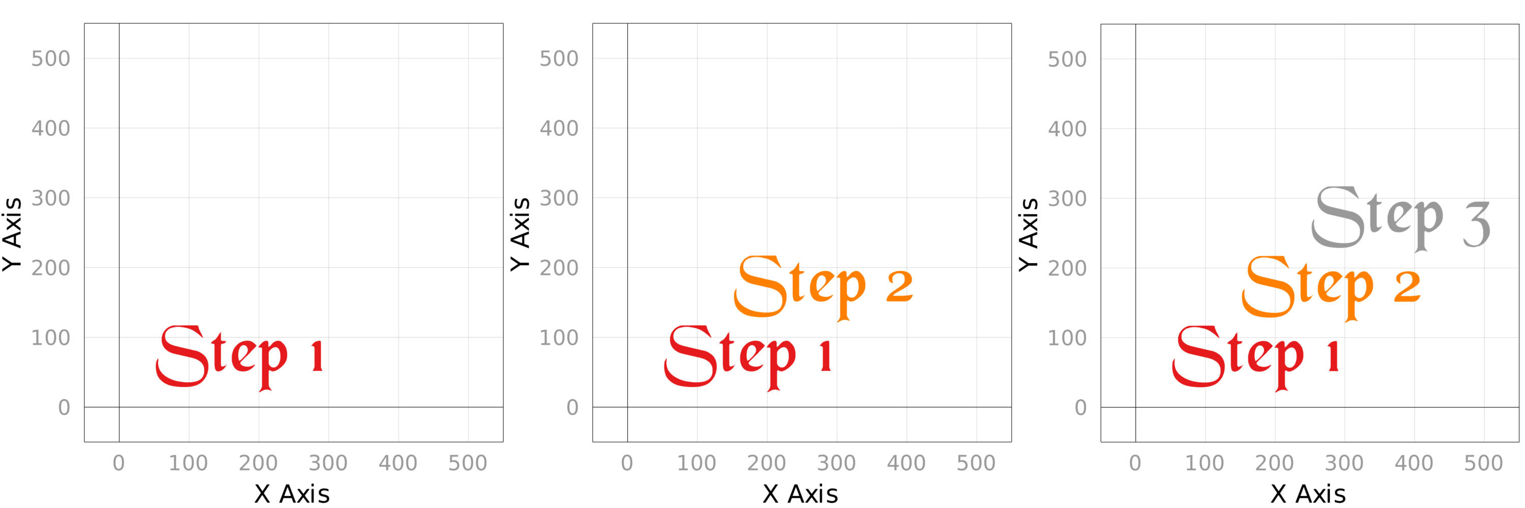
Stepper plots were also created, which are great for showing off progressive changes in plots, such as demonstrating the effects of theming or changing data.
mutable struct Stepper
  scene::Scene
  folder::String
  step::Int
end

function step!(s::Stepper)
  Makie.save(joinpath(s.folder, basename(s.folder) * "-$(s.step).jpg"), s.scene)
  s.step += 1
  return s
end
Creating and saving a stepper plot:
scene = Scene()
# text annotation
steps = ["Step 1", "Step 2", "Step 3"]
# initialize the stepper and give it an output destination
st = Stepper(scene, @outputfile)
for i = 1:length(steps)
  text!(
    scene,
    steps[i],
    scale_plot = false
  )
  step!(st) # saves the step and increments the step by one
end
For each step!(st), a new plot snapshot is saved.
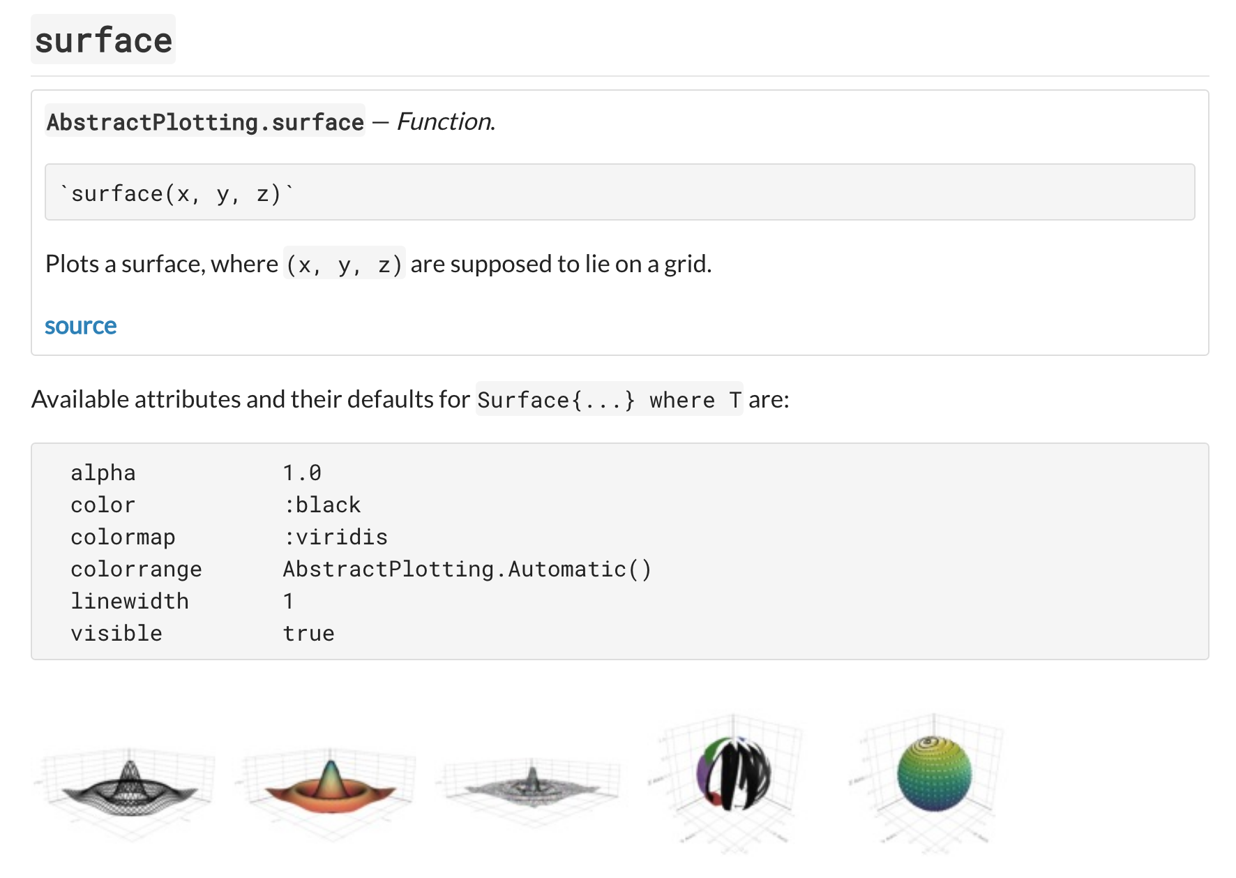
Implement overview page for plotting functions with example plots
This was achieved by iterating through the plotting functions and generating the documentation using the help functions implemented earlier. The overview page shows the docstring of each of the plotting functions and the available plot attributes for the plot (plus default values).
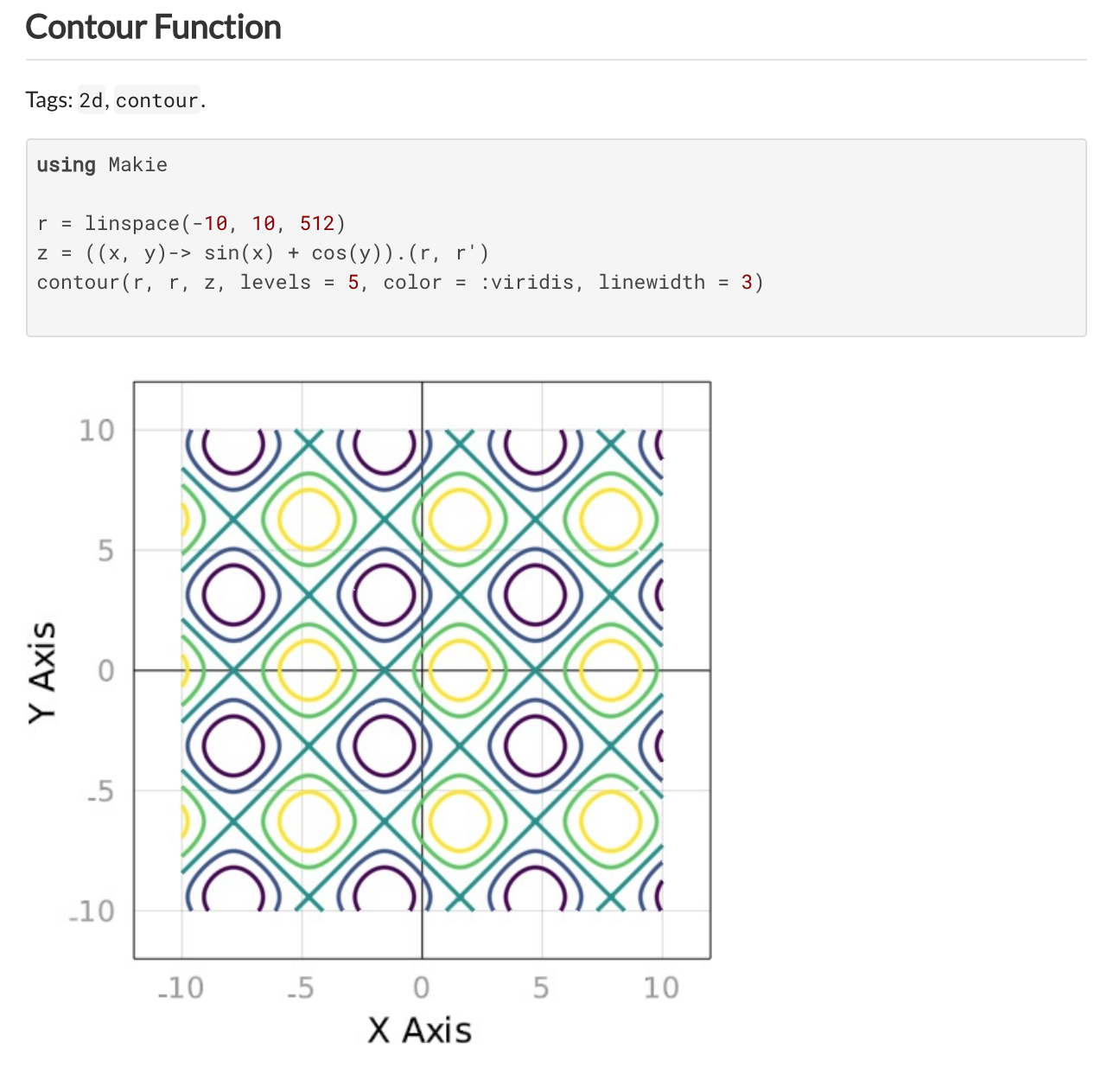
Implement preview gallery / categorical pages of plot types (e.g. all scatter plots)
This was achieved by iterating through the plotting functions and creating a separate page for each of the plotting functions. Then, all plots examples (including animated plots) of a given plotting function are inserted along with the source code to generate the plots.
An index page listing all of the examples pages and title of each example is also generated.
Substantially-automated documentation generation
A large part of the documentation generation is now automated.
The aim here is to reduce the amount of writing and manually updating of the documentation pages, whenever a code or recipe change is made. Thus, efforts are also made so that the docs generation mechanism is robust.
This is done by creating a base page for documentation pages, e.g. “src-axis.md” for mostly static text, and then adding dynamically-generated content to that to further generate an “axis.md” page which will eventually be compiled using Documenter.
The dynamically-generated content is different for each page. For axis.md, for example, it contains pretty-printed Markdown tables of the axis attributes, for 2D and 3D axes (all dynamically generated).
All example plots from the examples database are generated in one go initially (see the make.jl file), and given a unique name based on the example’s title. A thumbnail is also generated for each example. Later, the saved plot files are embedded into the example pages as needed.
Originally-submitted proposal
My proposal for Makie can be found on Google Docs.
![]() Image source: Google Summer of Code, CC BY-NC-ND 3.0
Image source: Google Summer of Code, CC BY-NC-ND 3.0